
Whether you are cleaning up a messy dataset, building a dynamic dashboard, or just trying to save a few hours of manual work, Excel’s modern formula toolkit has you covered. Here are 26 essential Excel formulas for 2026 based on Microsoft Office 365.
If you want to move past basic SUM and AVERAGE functions, here is a quick-reference guide to powerful formulas (function names and patterns) that will help you work smarter and faster.
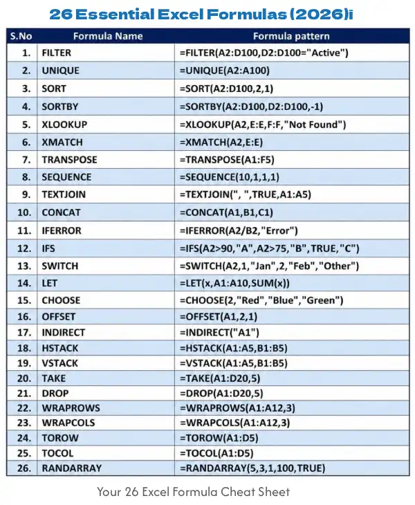
Table of Contents
26 Essential Excel Formulas for 2026
Dynamic Arrays & Sorting
These formulas automatically “spill” results into multiple cells, making data extraction incredibly seamless.
- FILTER: Extracts data that meets specific criteria.
- Pattern:
=FILTER(A2:D100, D2:D100="Active")
- UNIQUE: Returns a list of unique values from a range by removing duplicates.
- Pattern:
=UNIQUE(A2:A100)
- SORT: Sorts a range or array based on a specific column.
- Pattern:
=SORT(A2:D100, 2, 1)
- SORTBY: Sorts a range based on the values in a separate, corresponding range.
- Pattern:
=SORTBY(A2:D100, D2:D100, -1)
Advanced Lookups
Say goodbye to the limitations of old-school lookups. These formulas find exactly what you need, wherever it lives.
- XLOOKUP: The modern successor to VLOOKUP. It searches a range for a match and returns the item from another range.
- Pattern:
=XLOOKUP(A2, E:E, F:F, "Not Found")
- XMATCH: Returns the relative position of an item in an array or range.
- Pattern:
=XMATCH(A2, E:E)
Text & Data Formatting
Manipulating strings and rearranging layouts doesn’t have to be tedious.
TRANSPOSE: Flips the orientation of a range from vertical to horizontal (or vice versa).
Pattern: =TRANSPOSE(A1:F5)
- SEQUENCE: Generates a list of sequential numbers in an array.
- Pattern:
=SEQUENCE(10, 1, 1, 1)
- TEXTJOIN: Combines text from multiple ranges using a specific delimiter (like a comma or space).
- Pattern:
=TEXTJOIN(" ", TRUE, A1:A5)
- CONCAT: Joins multiple text strings or ranges together.
- Pattern:
=CONCAT(A1, B1, C1)
Logic & Error Handling
Keep your spreadsheets clean, professional, and free of ugly error messages.
- IFERROR: Returns a custom value you specify if a formula evaluates to an error.
- Pattern:
=IFERROR(A2/B2, "Error")
- IFS: Checks multiple conditions and returns a value corresponding to the first true condition.
- Pattern:
=IFS(A2>90, "A", A2>75, "B", TRUE, "C")
- SWITCH: Evaluates an expression against a list of values and returns the first matching result.
- Pattern:
=SWITCH(A2, 1, "Jan", 2, "Feb", "Other")
Advanced Variables & References
For complex modeling, these functions offer high-level control over how data is calculated and referenced.
- LET: Assigns names to calculation results, making complex formulas easier to read and faster to run.
- Pattern:
=LET(x, A1:A10, SUM(x))
- CHOOSE: Returns a value from a list of choices based on an index number.
- Pattern:
=CHOOSE(2, "Red", "Blue", "Green")
- OFFSET: Returns a reference to a range that is a specified number of rows and columns from a cell.
- Pattern:
=OFFSET(A1, 2, 1)
- INDIRECT: Returns the reference specified by a text string.
- Pattern:
=INDIRECT("A1")
Array Stacking & Reshaping
Perfect for combining multiple data sources or restructuring layout formats instantly.
- HSTACK: Appends arrays horizontally (side-by-side) into a single array.
- Pattern:
=HSTACK(A1:A5, B1:B5)
- VSTACK: Appends arrays vertically (stacked on top of each other) into a single array.
- Pattern:
=VSTACK(A1:A5, B1:B5)
- TAKE: Keeps a specified number of contiguous rows or columns from the start or end of an array.
- Pattern:
=TAKE(A1:D20, 5)
- DROP: Removes a specified number of rows or columns from the start or end of an array.
- Pattern:
=DROP(A1:D20, 5)
- WRAPROWS: Wraps a row or column of values into a 2D array by rows after a specified number of elements.
- Pattern:
=WRAPROWS(A1:A12, 3)
- WRAPCOLS: Wraps a row or column of values into a 2D array by columns after a specified number of elements.
- Pattern:
=WRAPCOLS(A1:A12, 3)
- TOROW: Flattens an entire array or range into a single row.
- Pattern:
=TOROW(A1:D5)
- TOCOL: Flattens an entire array or range into a single column.
- Pattern:
=TOCOL(A1:D5)
Randomization
- RANDARRAY: Generates an array of random numbers based on specified rows, columns, minimums, maximums, and data types.
- Pattern:
=RANDARRAY(5, 3, 1, 100, TRUE)
Pro Tips: Bookmark this guide or save the formula patterns so you can copy, paste, and adjust the cell references to match your own datasets the next time you’re stuck!
Conclusion
You don’t need to be an Excel expert to work smarter. These 26 formulas represent the most powerful tools available in modern Excel 365 — whether you’re cleaning messy datasets, building dynamic dashboards, or automating repetitive tasks. The shift from static formulas to dynamic arrays, intelligent lookups, and advanced text manipulation means you can accomplish in minutes what used to take hours of manual work.
The best part? Most of these functions work seamlessly together. Once you master a few core patterns — like FILTER for data extraction or XLOOKUP for finding values — you’ll start recognizing where other formulas fit naturally into your workflow.
Start with one formula that solves your most pressing problem today. Copy the pattern, adjust the cell references, and experiment. You’ll quickly discover which formulas become your go-to tools. Bookmark this guide, share it with your team, and watch your productivity soar.