Dynamic filters in Excel automatically adjust your data view as information changes, so you don’t have to manually re-filter every time something updates. Instead of clicking through filter options repeatedly, you set up a formula once and it handles the heavy lifting for you.

Excel Dynamic Filters is especially handy if you’re working with data that shifts frequently —sales figures, inventory levels, or employee metrics — and you need reports that always show the latest picture without extra work.

How Dynamic Filters Actually Works?

The magic happens through formulas, particularly the FILTER() function. Once you plug in a FILTER formula, it creates a live list that updates automatically whenever your source data changes.

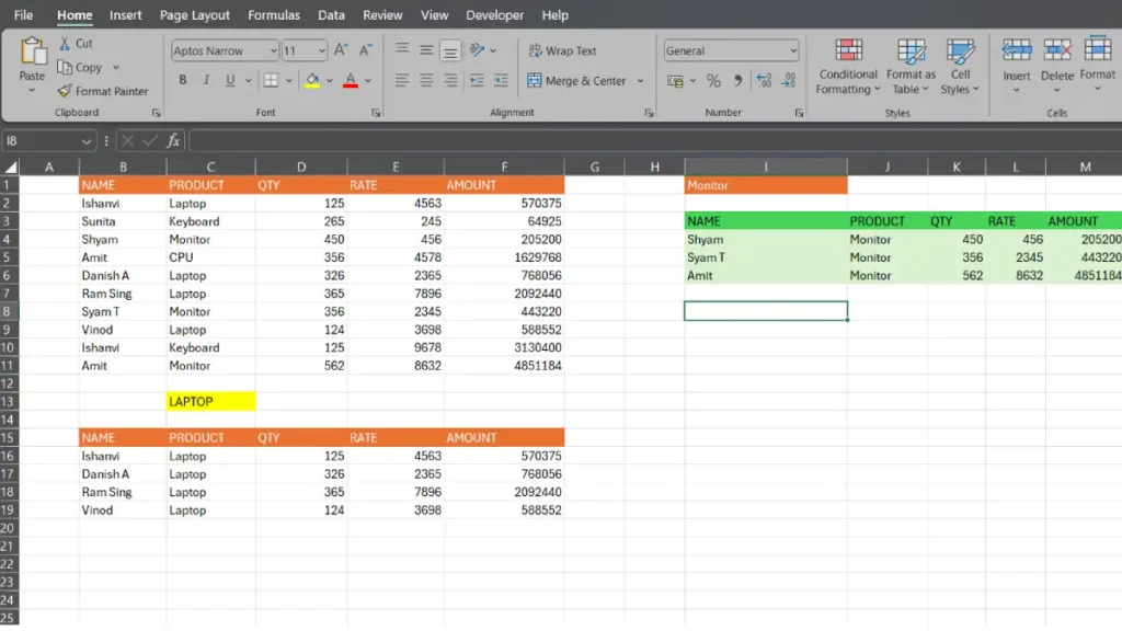
Here’s a practical example: imagine you have a sales table and want to see how many times a specific product has sold. Set up the right formula, and every time a new sale gets added to your dataset, that filtered view updates instantly — no manual intervention needed.

A basic formula looks like this: =FILTER(B2:F11, C2:C11=C13) where B2:F11 is your sales data, C2:C11 is the items sold column, and C13 is the cell where you enter the product name you want to filter by.

Setting Up Your First Dynamic Filter in Excel

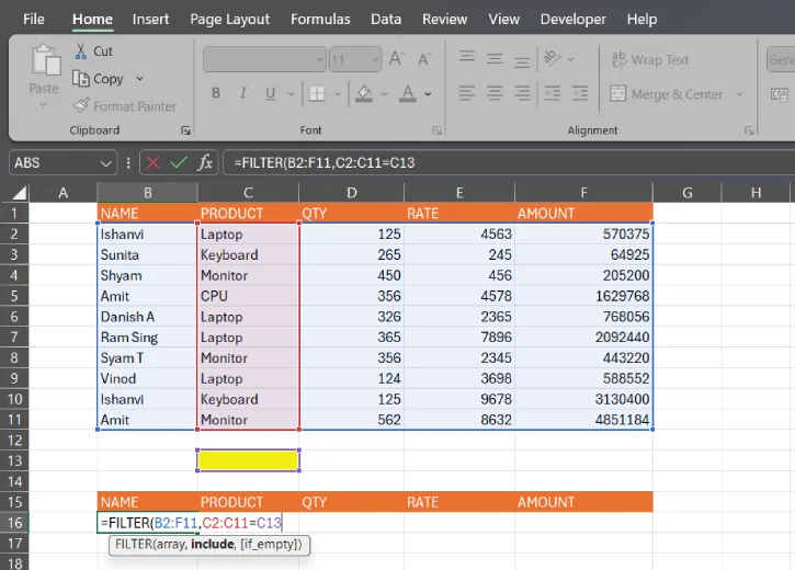
1. Getting started is straightforward. Enter your FILTER formula into a cell, then press Enter. Using the sales example above:

• B2:F11 = your complete sales dataset (adjust these cell references to match your actual data)
• C2:C11 = the column listing items sold
• C13 = where you’ll type in the product name you want to look up

2. Type a product name in that designated cell, and boom — you immediately see results for that item. Add a new sale to your dataset, and the filtered results update on their own.

Note: FILTER() function is available in: Excel 365 (all current subscriptions), Excel 2021 and newer and Excel Online (web version)

How to Combine FILTER() With Other Functions for Advanced Dynamic Filtering?

Once you’re comfortable with basic dynamic filters, you can combine them with other functions for even more powerful reporting. Here are three combinations that work great:

1. FILTER() + SORT()

Want your filtered results sorted automatically? Wrap your FILTER formula inside SORT():

=SORT(FILTER(B2:F11, C2:C11=C13), 2, FALSE)

This filters your data, then sorts it by the second column in descending order. Perfect for showing top-selling items first.

2. FILTER() + UNIQUE()

If your dataset has duplicates and you only want to see each item once, nest UNIQUE inside FILTER():

=UNIQUE(FILTER(B2:F11, C2:C11=C13))

Now your filtered list shows each product only once, even if it appears multiple times in your source data.

3. FILTER() + COUNTA()

Need a quick count of how many rows match your filter criteria? Pair it with COUNTA():

=COUNTA(FILTER(B2:F11, C2:C11=C13))

This tells you exactly how many items meet your filter condition — handy for inventory or sales summaries.

These combinations sound fancy, but they’re just building blocks. Start with basic FILTER(), and once that feels natural, experiment with adding SORT or UNIQUE. Your reports will go from useful to impressive.

ALSO READ: You’re Using Excel Wrong: Learn These 5 Paste Special Features

Troubleshooting Common Issues

When you first set up a dynamic filter, things don’t always work smoothly. Here are the most common problems and how to fix them:

Wrong Cell References

The most common mistake is copying a formula without updating the cell ranges to match your actual data. If you use the example formula =FILTER(B2:F11, C2:C11=C13) but your sales data starts in row 3 instead of row 2, the formula will either skip data or pull empty rows. Double-check that your first number matches where your data actually begins, and the second number matches where it ends.

Text vs. Numbers Mismatch

Excel gets picky when you filter text as numbers (or vice versa). If you’re filtering product names but accidentally entered numbers in your criteria cell, the filter returns nothing. Make sure the data type in your criteria cell matches what you’re filtering. If your product names are text, enter them as text. If you’re filtering by ID numbers, use numbers.

Formula Shows #REF! Error

This usually means you deleted a column or row that the formula references. Go back and check — did you remove the column your criteria cell was in? Rebuild the formula with the correct current cell references.

Results Update Slowly

If your spreadsheet has thousands of rows and the filter lags, it’s not broken, it’s just a lot of work for Excel. Consider splitting your data into smaller ranges or using a pivot table for massive datasets. Dynamic filters work best with datasets under 10,000 rows.

Conclusion

Dynamic filters in Excel automate data management across sales, inventory, HR, and finance by automatically updating reports without manual intervention. This approach enables real-time reporting, reduces errors, eliminates busywork, accelerates decision-making, and scales effortlessly as data grows — allowing teams to focus on analysis rather than spreadsheet maintenance.