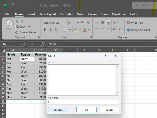
In Excel Ctrl+G is probably the most underused shortcut – but it’s hiding one of the platform’s most powerful data cleanup tools. Press it, click Special, and unlock advanced cell selection features that would normally require digging through menus or writing helper formulas.

If you work with Excel data cleanup, Ctrl + G is a real time-saver. You don’t need to go through Home tab, and hunting for the cleanup tools, you can just hit Ctrl + G and you’re there in seconds. Here are 5 data cleanup tricks using this shortcut.

Benefits of Using Ctrl+G in Excel

1. Select all blank cells at once: Identify and delete empty rows in seconds, even on sheets with thousands of rows, without manually selecting each one.

2. Highlight all formulas simultaneously: Visually distinguish calculated cells from hardcoded inputs by selecting every formula in your range, then apply formatting to make them stand out.

3. Isolate formula errors quickly: Filter to show only broken formulas (using the Errors sub-filter) so you can fix problems without wrapping every calculation in IFERROR.

4. Select all hardcoded values: Use the Constants option to audit your raw inputs separately from your calculations.

5. Copy filtered or hidden data cleanly: Select only visible cells to ensure hidden rows don’t accidentally tag along when you copy and paste, especially with grouped or outlined data.

6. Find inconsistencies without helper formulas: The Row Differences option highlights cells that break the pattern of their neighbors, providing a quick consistency check.

7. Bulk-select comments and objects: Select every annotated cell at once (useful for stripping markup before sharing) or every image, chart, and shape on your sheet (faster than clicking through individually).

Below are 5 Excel data cleanup tricks – delet blank rows, find and fix formula errors, copy filtered data without dragging hidden rows, highlight all formulas to distinguish them from raw data, bulk select all comments before sharing a Workbook – using the Excels’ Ctrl + G shortcut.

ALSO READ: How to Hide Zero Values in Excel Instantly: Two Quick Methods

How to Use Ctrl+G in Excel: Step-by-Step Examples

Example 1: Delete Blank Rows from a Dataset

Scenario: You have a sales file with 33 rows of data followed by hundreds of empty rows.

• Select the column you want to scan for blanks (e.g., the Salesperson column as an anchor point).
• Press Ctrl+G, then click the Special button.
• Choose Blanks and click OK — Excel highlights every cell with a missing value in that column.
• Right-click any highlighted cell and select Delete > Entire row.

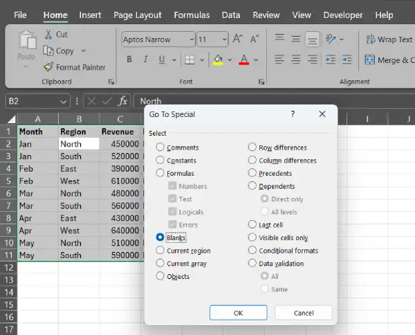
Result: All blank rows are removed in seconds, even on a 6,000-row sheet.

Example 2: Highlight All Formulas to Distinguish Them from Raw Data

Scenario: You have a Commission and Profit Margin column with formulas, but they look identical to hardcoded numbers. You want to make formulas visually distinct so mistakes stand out.

• Select the range containing your data.
• Press Ctrl+G, then click Special.
• Choose Formulas and click OK — every cell containing a formula is highlighted.
• Right-click the highlighted cells and apply a fill color (e.g., light blue or yellow).

Result: Formulas now stand out visually from raw inputs, making accidental overwrites obvious.

Example 3: Find and Fix Formula Errors

Scenario: Your spreadsheet has multiple formulas, and you know some are broken, but you can’t spot which ones by eye.

• Select your data range.
• Press Ctrl+G, then click Special.
• Choose Formulas, then click OK.
• From the resulting menu, narrow it further to Errors to isolate only broken formulas.

Result: Only cells with formula errors are selected, so you can fix them directly without searching manually or wrapping every formula in IFERROR.

Example 4: Copy Filtered Data Without Dragging Hidden Rows

Scenario: You’ve manually hidden rows for regions you don’t want (e.g., collapsed South and East regions), and now you want to copy only the visible North and West data to send to a colleague.

• Hide or collapse the rows you don’t need to see.
• Select the visible range you want to copy.
• Press Ctrl+G, then click Special.
• Choose Visible cells only and click OK.
• Copy (Ctrl+C) and paste the selection elsewhere.

Result: Only the visible rows transfer — hidden rows don’t accidentally tag along, which is especially important with grouped or outlined data.

Example 5: Bulk-Select All Comments Before Sharing a Workbook

Scenario: You’ve added internal notes and comments throughout a spreadsheet, but now you need to strip them before sending the file to a client.

• Select your entire data range (or the sheet).
• Press Ctrl+G, then click Special.
• Choose Notes (or Comments) and click OK — every annotated cell is selected.
• Right-click and delete the selected comments, or use the Review tab to remove them in bulk.

Result: All markup is removed at once instead of clicking through each comment individually.

Conclusion

Ctrl+G transforms tedious spreadsheet maintenance into seconds of work. Master these five techniques, and you’ll never manually hunt through data the same way again