How to Hide Zero Values in Excel Instantly: Two Quick Methods

Hiding zero values in Excel can instantly clean up your spreadsheet and make it easier to focus on data that really matters. Whether you’re working with calculations that frequently result in zero or just want a cleaner visual presentation, Excel offers straightforward methods to hide zeros temporarily or permanently.

There are several ways to hide or remove zero value from spreadsheet. This guide explains two methods to hide zero values in selected or range of cells. You can quickly hide zeroes in cells where it’s the only number (and where the formula within the cell results in zero).

Table of Contents

Two Methods to Hide Zero Values in Excel Quickly

Method 1: Using Format Cells to Hide Zeros

This is the quickest way to hide zeros in selected cells and works for both existing data and future entries in that range.

1. Select the cells containing the zero values you want to hide.

2. Open the Format Cells dialog using one of these options:

Press Ctrl+1 (fastest method)
Click Home tab > Format > Format Cells
Right-click the cell and select Format Cells

3. Navigate to the Number tab and select Custom from the category list at the bottom.

4. Enter the custom format code: In the Type box, type 0;-0;;@ and click OK.

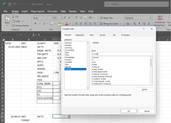
Instantly hide zeros in Excel spreadsheet

5. Cells containing only zeros will now appear blank

6. To restore the zeros later, repeat steps 1–3 and type 0;-0;0;@ instead, then click OK.

Method 2: Using Conditional Formatting for Dynamic Worksheets

If your Excel sheet is constantly updated and you want to prevent zeros from appearing automatically, Conditional Formatting is your best option.

1. Select the range of cells where you want to hide zeros.

2. Go to the Home tab and click Conditional Formatting > New Rule.

3. Set up the rule:

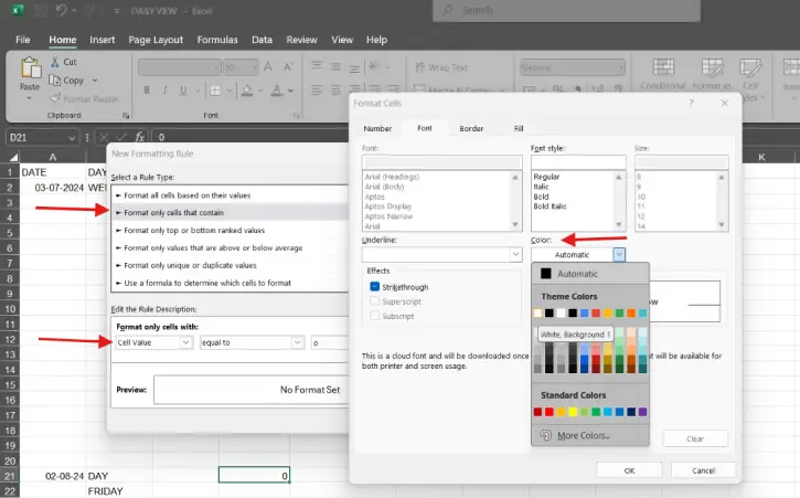
Change the rule type to “Format only cells that contain“
Select Cell Value
Choose equal to
Enter 0 in the value box
Set the formatting: Click Format and choose a font color that matches your cell background (typically white), or set the font color to be invisible.

Use conditional formating to hide zeros from Excel spreadsheet

4. Click OK to apply the rule to your selected range.

Final Thought

Hiding zeros in Excel is a simple way to improve readability and focus attention on the data that matters most. Choose Format Cells for quick, one-time formatting of existing data, or opt for Conditional Formatting if you’re working with a dynamic spreadsheet that’s regularly updated. Both methods preserve your data while giving you cleaner, more professional-looking results. Try whichever method suits your workflow best, you can always undo it if needed!