
Still using Excel the slow way? These 6 Excel shortcuts will save you hours every week. Excel shortcuts let you perform certain tasks instantly, eliminating the need to navigate through menus and click multiple times. Stop wasting time navigating menus. Here are the six shortcuts that separate Excel power users from everyone else.
These six shortcuts can cut your spreadsheet work time in half—even if you’re already comfortable with Excel. Below are the Excel shortcuts and their real-world examples.
Ctrl + t : Insert table
Ctrl + \ : Select differences
Ctrl + q : Quick analysis
Alt + = : 1-second sum
Alt + F1 : Create chart
Alt + Enter : Line break
Table of Contents
6 Most Useful Excel Shortcuts, Their Explanations and Real-World Examples
1. Ctrl + T: Insert Table
Ctrl + T converts a range of data into a formatted table with automatic headers, alternating row colors, and filter buttons. This makes your data more organized and easier to work with.
Real-World Example:
You have a list of 200 customer names, emails, and purchase amounts in columns A, B, and C. Instead of manually formatting each row, you:
- Select your data range (A1:C200)
- Press Ctrl + T
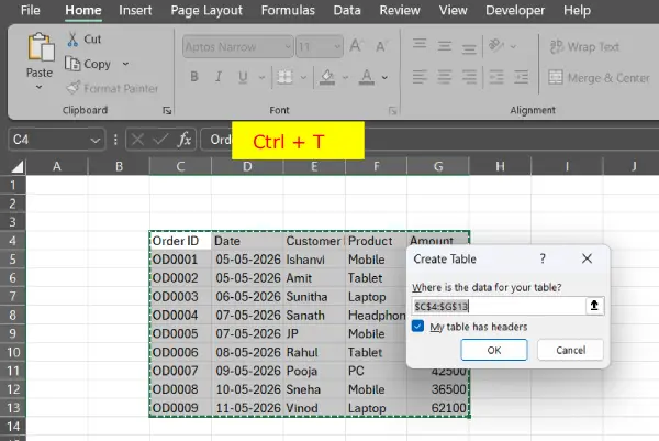
Excel instantly creates a professional table with blue headers, alternating row shading, and dropdown filters on each column header
Now you can sort customers by purchase amount or filter by specific names without affecting other data—something much harder with plain cells.
2. Ctrl + \: Select Differences
Ctrl + \ highlights cells that differ from the first cell in your selection, helping you spot inconsistencies or errors in similar data.
Real-World Example:
You’re auditing a spreadsheet where column A should contain identical product codes (all should be “PROD-001”). You:
- Select the range A2:A50
- Press Ctrl + \
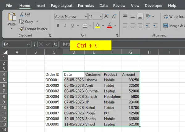
Excel highlights any cells that don’t match A2, immediately showing you that row 15 has “PROD-002” and row 32 has a typo “PROD-001 “
This saves hours of manual comparison in quality control or data validation tasks.
3. Ctrl + Q: Quick Analysis
Ctrl + Q opens the Quick Analysis toolbar, which suggests charts, formulas, conditional formatting, and totals based on your selected data.
Real-World Example:
You have monthly sales data (January–December revenue) in cells B1:M1, and you want to visualize the trend. You:
- Select your data range
- Press Ctrl + Q
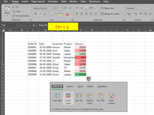
The Quick Analysis panel appears with chart recommendations—you see a line chart preview showing your revenue trend
Click the suggested line chart, and it’s created instantly. Instead of manually building formulas or navigating menus, Excel intelligently offers exactly what you need in seconds.
ALSO READ: Understanding the Excel IF Function: A Simple 3-Part Guide
4. Alt + =: 1-Second Sum
Alt + = instantly inserts a SUM formula for the cells above or to the left of your current cell, making quick calculations effortless.
Real-World Example:
You have quarterly revenue figures in cells B2:B5, and you need a total in B6. You:
- Click cell B6
- Press Alt + =
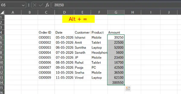
Excel automatically inserts =SUM(B2:B5) and displays the total
This is especially useful in financial reports where you might add totals for dozens of columns—much faster than typing formulas manually.
5. Alt + F1: Create Chart
Alt + F1 instantly creates a default chart from your selected data without opening dialog boxes. The chart appears as an object on your worksheet.
Real-World Example:
You’re building a presentation and have sales data for three regions (North, South, West) with quarterly figures. You:
- Select your data including headers (A1:D4)
- Press Alt + F1
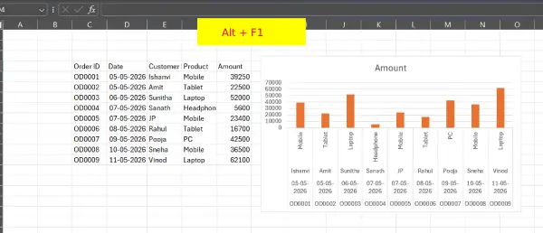
Excel creates a column chart immediately on the same sheet showing all three regions across quarters
You can then resize, reposition, or customize the chart as needed—but the time-consuming part is already done.
6. Alt + Enter: Line Break
Alt + Enter inserts a line break within the same cell, allowing you to display multiple lines of text in a single cell without creating multiple rows.
Real-World Example:
You’re creating a project management sheet and need to list multiple tasks within a single cell for a project phase. In cell A1, you want to show:
Design mockups
Client review
Revisions
You:
- Type “Design mockups”
- Press Alt + Enter
- Type “Client review”
- Press Alt + Enter
- Type “Revisions”
- Press Enter to confirm
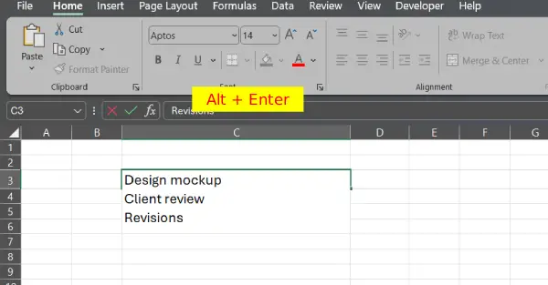
Now all three items appear stacked within one cell instead of spreading across three rows, keeping your data compact and readable. (Make sure to set the cell to “Wrap Text” so all lines are visible.)
Conclusion
Whether you’re formatting data with Ctrl + T, spotting errors with Ctrl + \, or creating charts in seconds with Alt + F1, these keyboard combinations eliminate repetitive clicking and keep you focused on what matters. The beauty of Excel shortcuts is that they compound—each one saves just a few seconds, but across hundreds of spreadsheets and thousands of tasks throughout your career, those seconds add up to days of reclaimed time. Start with the shortcuts that fit your daily workflow, practice them until they become muscle memory, and gradually integrate the others. Your future self—and your deadline-driven projects—will thank you.