We’ve all been there—you’re building out a Google Sheets spreadsheet, everything’s looking good, and then suddenly: #ERROR! or #REF! stares back at you from a cell. This formula parse errors are frustrating, especially when the error message tells you nothing useful.

The good news? Most Google Sheets formula errors – ERROR, #N/A, #REF, #VALUE, #NAME and #NUM – are pretty easy to fix once you understand what they mean.

Important: Note that the integration of Gemni in Sheets now lets you figureout the formula parse errors easily.

What’s a Formula Parse Error, Anyway?

A formula parse error simply means Google Sheets can’t understand the instructions you’ve given it. Think of it like sending a text message with a bunch of typos—the other person gets confused because they can’t make sense of what you’re saying.

Here’s a real example: Let’s say you want to pull data from another sheet called “Sheet1,” so you write this formula: =Sheet1!A1

That exclamation mark is crucial. It tells Google Sheets you’re looking in a different sheet. But if you accidentally type =Sheet1A1 (missing the !), Google Sheets throws up its hands and says “I don’t understand this.”

The handy part? Google Sheets usually categorizes the error for you—#REF!, #VALUE!, #NAME?, and so on. These error codes are like breadcrumbs that help you figure out what went wrong.

The Most Common Formula Errors (And How to Fix Them)

#ERROR! – The Unhelpful One

Let’s start with the most annoying error: #ERROR! This is the spreadsheet equivalent of getting a shrug emoji as a response. When you hover over it, Google Sheets just says “Formula parse error”—which… yeah, you already knew that.

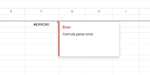
Fix: Unfortunately, there’s no shortcut here. You’ll need to carefully go through your formula, element by element, checking for typos, missing symbols, or invalid references. It’s tedious, but it works.

Pro tip: Start from the beginning of your formula and work your way through. Check for missing colons, parentheses, quotation marks, or special characters.

#N/A – The “Value Missing” Error

You’ll see #N/A when Google Sheets can’t find the value you’re asking it to look for. This happens most often when you’re using lookup functions like VLOOKUP or INDEX/MATCH.

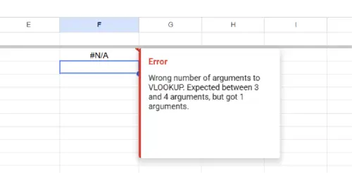
For example, imagine you’re using an INDEX/MATCH formula to find someone’s salary, but you reference a cell (like C17) that’s actually empty. Google Sheets can’t find the data, so it returns #N/A.

How to fix it:

• Double-check that the cell you’re referencing actually contains data
• Make sure you’re looking in the right range
• Verify that the lookup value exists somewhere in your reference data

#REF! – The “Cell Doesn’t Exist” Error

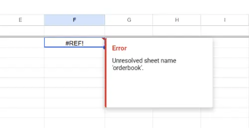
The #REF! error means your formula is trying to reference a cell that no longer exists. Usually, this happens because someone deleted a cell or an entire column.

Example scenario: You create a formula like =SUM(A2:D2) in cell F2. Then you delete column C. Now your formula is confused because one of the cells it was supposed to reference is gone.

How to fix it:

Option 1 – Undo the deletion: If you just deleted something and got this error, immediately press Ctrl+Z (or Cmd+Z on Mac) to undo.

Option 2 – Update your formula: Change your formula to use a cell range instead of individual cell references. For some reason, Google Sheets handles ranges better when cells go missing. So instead of referencing specific cells separated by commas, use ranges like A1:D1.

Option 3 – Use absolute references: This one’s a bit more advanced, but it’s super helpful if you’re copying formulas around your sheet.

When you copy a formula to a new location, Google Sheets automatically adjusts the cell references to match the new position. That’s called a relative reference, and it usually works great. But sometimes it causes problems.

For example, if you copy =SUM(A2:A7) from cell F2 and paste it way down in cell F5, Google Sheets thinks you want to sum the six cells above F5. But there might only be three cells available, so—error!

The fix? Make your references absolute by adding dollar signs. Change =SUM(A2:A7) to =SUM($A$2:$A$7). Now, no matter where you copy the formula, it will always reference the exact same cells.

#VALUE! – The “Wrong Data Type” Error

VALUE! shows up when your formula is trying to do something with the wrong type of data.

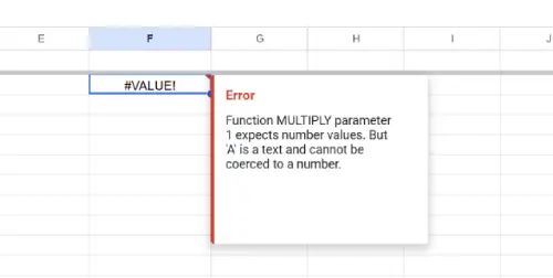
Real-world example: You’re trying to multiply two cells together with the formula =A1*F2. But cell F2 contains the text “five” instead of the number 5. Google Sheets can’t multiply a number by text, so it returns #VALUE!

How to fix it:

• Make sure cells being used in math operations contain actual numbers, not text
• If you need to convert text to numbers, you might need to use a different formula or function
• Double-check that you’re not mixing text and numbers in your calculations

#NAME? – The “Typo in Your Formula” Error

The #NAME? error usually means one of two things:

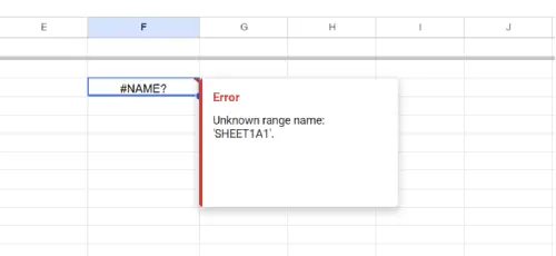
Problem 1 – You misspelled a function name

You meant to write =SUM(A1:A3) to add up those cells, but you accidentally typed =SUMM(A1:A3). That extra M throws everything off, and Google Sheets doesn’t recognize “SUMM” as a real function.

How to fix it: Correct the spelling. The good news is that Google Sheets will try to autocomplete function names as you type, so use that feature to avoid typos.

Problem 2 – You forgot quotation marks around text

Some formulas need you to wrap text in quotation marks. For example, if you want to join two text strings together, you’d use:

=CONCATENATE("Bur","rito")

But if you forget the quotation marks around “rito” and write:

=CONCATENATE("Bur",rito)

Google Sheets thinks “rito” is a named range or function, can’t find it, and returns #NAME?

How to fix it: Add quotation marks around any text strings in your formula.

#NUM! – The “Invalid Number” Error

NUM! pops up when your formula tries to do something mathematically impossible (or at least, impossible for Google Sheets to display).

Common scenarios:

• Your formula asks Google Sheets to find the square root of a negative number (the answer isn’t a real number)
• Your formula tries to generate a number so large that Google Sheets can’t display it
• You’re using a function with a value outside its acceptable range

How to fix it:

• Hover over the error message—Google Sheets usually gives you more details about what went wrong
• Adjust your formula based on that description
• If you’re using square roots, make sure you’re working with positive numbers
• Check that any numbers you’re plugging into functions fall within reasonable ranges

The Bottom Line

Formula errors in Google Sheets aren’t a sign you’re doing something fundamentally wrong. They’re just Google Sheets’ way of saying “Hey, I don’t understand what you’re asking me to do.” Once you know what each error code means, you can track down the problem and fix it quickly.

The most common culprits? Typos, missing symbols (like ! or :), deleted cells, and mixing text with numbers. Check those first, and you’ll solve most of your formula headaches.