

Let me break down VLOOKUP for you in a way that actually makes sense. Sure, you could ask Google Sheets‘ built-in Gemini AI to write the formula for you, but here’s the thing—if something goes wrong (and it will eventually), you’ll be stuck. Understanding how VLOOKUP works means you can troubleshoot it yourself and use it confidently.
Table of Contents
What’s VLOOKUP, Really?
VLOOKUP or vertical lookup in Google Sheets is your spreadsheet’s search-and-retrieve tool. It helps you find a value you’re looking for in one column, then grabs related information from another column in the same row.
This is gold when you’re dealing with huge datasets. Imagine a spreadsheet with thousands of students, their ID numbers, and departments. Instead of manually hunting through it all, VLOOKUP instantly pulls exactly what you need.
Here’s how it works in simple terms:
- You have data: A table with rows and columns full of information
- You want something: A specific piece of data, like a student ID or name
- VLOOKUP finds it: It searches for your target value in one column
- VLOOKUP returns it: It grabs the corresponding info from another column
The VLOOKUP Formula: Breaking It Down
Here’s what the formula looks like:=VLOOKUP(search_key, range, index, [is_sorted])
Let me explain each part so you know exactly what you’re doing:
- search_key – The value you’re hunting for (like a name or ID number)
- range – The section of your spreadsheet where the data lives (must include at least two columns)
- index – Which column number (within your range) contains the data you want back. If ages are in the 3rd column of your range, your index is 3.
- is_sorted – Whether your data is alphabetically or numerically sorted (TRUE or FALSE)
Why the is_sorted Matters
This is where people get tripped up. When you set is_sorted to TRUE, Google Sheets assumes your data is sorted A–Z or smallest to largest. It’ll search faster, but here’s the catch—it finds the closest match that’s less than or equal to your search value, not necessarily an exact match.
Set is_sorted to FALSE, and Google Sheets will dig deeper to find an exact match. If it can’t find one, you’ll get an #N/A error instead, which is actually helpful because it tells you something’s wrong.
How to Actually Use It: Step by Step
The easiest way? Ask Gemini in plain language. But let’s say you want to do it yourself. Here’s how:
Setting up a simple example
Let’s use a real scenario: you have a list of students and their ID numbers, and you need to find a specific student’s ID.
Step 1: Click the cell where you want your answer to appear (let’s say cell D5)
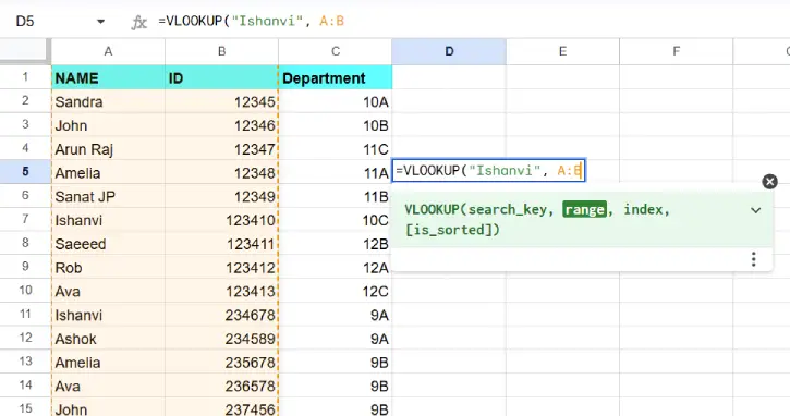
Step 2: Type in your VLOOKUP formula. Here’s what it might look like:=VLOOKUP("Ishanvi", A:B, 2, FALSE)
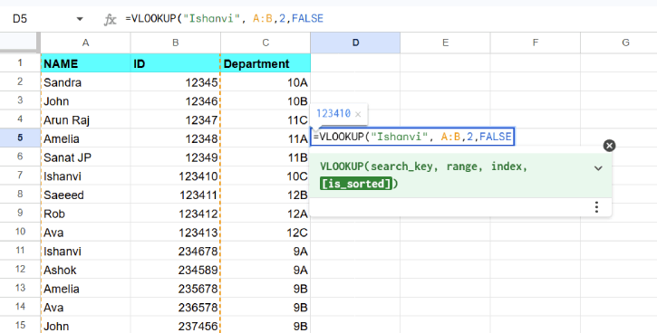
Let’s decode this:
- “Ishanvi” = the student’s name you’re looking for
- A:B = your table (column A has names, column B has IDs)
- 2 = you want the value from the 2nd column (the ID numbers)
- FALSE = you want an exact match, not an approximate one
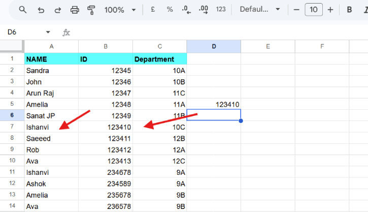
Step 3: Press Enter. If everything’s set up right, you’ll see Sarah’s employee ID pop up instantly.
ALSO READ: ChatGPT Prompts for Business Dashboards in Google Sheets
When VLOOKUP Goes Wrong (And How to Fix It)
It’s returning the wrong value
This usually means is_sorted is set to TRUE when it shouldn’t be. Check if your first column is actually sorted A–Z or numerically from smallest to largest. If it’s not, change it to FALSE. Simple as that.
It’s only giving you the first match
By design, VLOOKUP stops at the first match it finds. If you have multiple “Ishanvi” in your list, VLOOKUP will always grab the first one. The solution? Make your search unique by combining columns (more on this below).
Your data’s a mess
Extra spaces and typos kill VLOOKUP. If your lookup value has a space that the data doesn’t (or vice versa), no match. Before you start, clean up your spreadsheet. Go to Data > Data Cleanup > Trim whitespace to automatically remove unwanted spaces.
You’re getting #N/A errors
This means VLOOKUP couldn’t find an exact match. Double-check that your search value exists in the first column of your range, and make sure there are no hidden spaces or typos causing problems.
How to Search with Multiple Criteria
Here’s where it gets interesting. Let’s say you have multiple students named “Sanat JP,” and you need to distinguish between them using more than one piece of information.
The trick? Create a helper column that combines two values, then search for both at once.
Here’s how:
1. Add a helper column to the left of your lookup data. This becomes your new leftmost column.
2. In the first row of this column (say, A2), enter: =B2 & ” ” & C2 This formula joins the values from columns B and C with a space between them—so “Sanat” and “JP” become “Sanat JP.”
3. Copy that formula down the entire helper column.
4. Now use VLOOKUP with both criteria combined. For example:=VLOOKUP("Sanat JP", A2:D22, 4, FALSE)
5. This searches for “Sanat JP” (both values combined) in your helper column, then returns data from the 4th column of your range.
6. Adjust the numbers as needed. The range A2:D22 should include your helper column. The number 4 means you want the value from the 4th column—change it based on where your actual data is.
Conclusion
VLOOKUP is powerful once you understand what’s happening behind the scenes. Yes, AI can write it for you, but knowing how to set it up, troubleshoot it, and adapt it to different situations? That’s what makes you actually proficient with spreadsheets. Start simple, practice with small datasets, and you’ll be pulling data like a pro.

