
The QUERY function in Google Sheets is your Swiss Army knife for data manipulation. Instead of manually filtering and sorting through spreadsheets, you write a simple formula that does the heavy lifting for you. Sheets QUERY Function uses SQL-like commands—familiar to anyone who’s worked with databases—but right inside your Google Sheet.
Think of it this way: rather than clicking through menus and spending time on repetitive data wrangling, you can extract exactly what you need in one clean formula. It’s particularly useful when you’re working with large datasets and need to pull specific subsets of information for reports or dashboards.
Table of Contents
Google Sheets QUERY Function: Data Filtering & Analysis
Understanding the Syntax
The QUERY function follows this straightforward pattern:=QUERY(data, query, [headers])
Here’s what each part does:
- data: The range of cells containing your information (e.g., A2:D100). This is your source dataset.
- query: The SQL-like instruction that tells Google Sheets what to do—filter, sort, aggregate, or combine operations.
- headers: Optional parameter that indicates how many header rows exist (usually 1 if your first row contains column titles).
Setting Up Your Data
Before you write any QUERY formula, your data needs to be organized properly. Use a clean tabular structure with clear, descriptive column headers in the first row. Each column should contain a single type of information, and each row should represent a distinct record.
For example, if you’re tracking product sales, you might have:
- Column A: Product names
- Column B: Category
- Column C: Sales figures
- Column D: Date
This organization makes your queries cleaner and less error-prone.
Core QUERY Operations Explained
Selecting Specific Columns with SELECT
The SELECT clause lets you choose which columns to display in your results. You don’t need to show all columns—just pull the ones that matter.
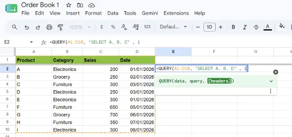
=QUERY(A1:D10, "SELECT A, B, C", 1)
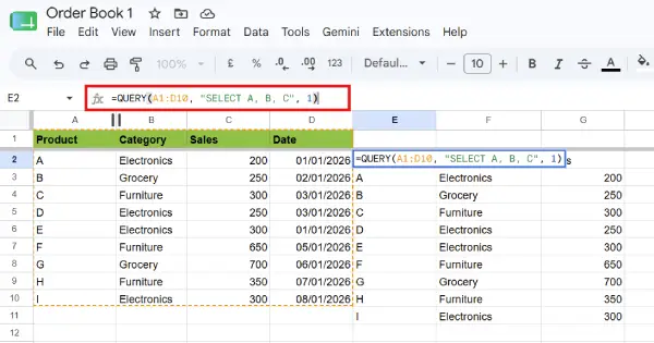
This grabs only the Product, Category, and Sales columns, leaving out Date entirely.
Filtering Data with WHERE
WHERE is your filter. It narrows down your results to only rows that match your criteria. You can use comparison operators like =, >, <, >=, <=, and combine conditions with AND or OR.
=QUERY(A2:D10, "SELECT A, C WHERE B = 'Electronics' AND C > 200")
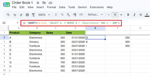
This pulls products and sales figures only for items in the Electronics category that sold more than 200 units.
Sorting with ORDER BY
ORDER BY arranges your results in ascending or descending order based on any column. Use ASC for ascending (the default) or DESC for descending.=QUERY(A2:D10, "SELECT A, C ORDER BY C DESC")
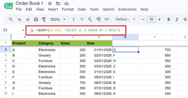
This shows products and sales sorted from highest to lowest sales.
Grouping & Aggregating Data with GROUP BY
GROUP BY is powerful for summarizing data. Combine it with aggregate functions like SUM, AVG, COUNT, MAX, or MIN to create summaries.=QUERY(A2:D10, "SELECT B, SUM(C) GROUP BY B")
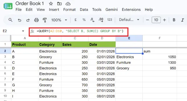
This totals sales by category, giving you a quick breakdown of performance across product types.
Limiting Results with LIMIT
LIMIT restricts how many rows you get back. This is handy when you only need the top performers or a sample of data.
=QUERY(A1:D10, "SELECT A, B, C, D ORDER BY C DESC LIMIT 3", 1)
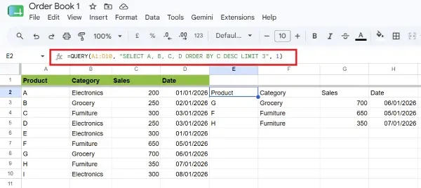
This shows just the three best-selling products.
Renaming Columns with LABEL
LABEL makes your output more readable by renaming columns. Instead of seeing “SUM(C)” in your results, you can call it something meaningful.=QUERY(A1:D10, "SELECT B, SUM(C) GROUP BY B LABEL SUM(C) 'Total Sales'", 1)
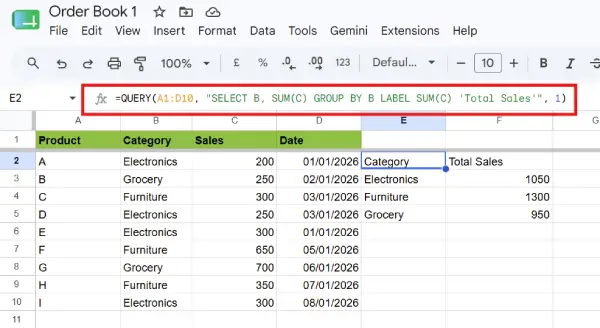
Now your aggregated column displays as “Total Sales” instead of the technical function name.
ALSO READ: Dynamic Filters in Google Sheets: Usage Guide With Example
Practical Examples You Can Use Now
| What You Want | Formula | Result |
| Top 2 Electronics products by sales | =QUERY(A1:D10, “SELECT A, C WHERE B = ‘Electronics’ ORDER BY C DESC LIMIT 2”, 1) | Shows the 2 best-selling electronics items |
| Total sales by category | =QUERY(A2:D10, “SELECT B, SUM(C) GROUP BY B LABEL SUM(C) ‘Total Sales'”) | Summarizes revenue for each product category |
| Products selling over 200 units | =QUERY(A2:D10, “SELECT A, C WHERE C > 200 ORDER BY C DESC”) | Lists high-performing products sorted by volume |
| All data sorted by date (newest first) | =QUERY(A1:D10, “SELECT A, B, C, D ORDER BY D DESC”, 1) | Chronological view with latest entries on top |
Combining Multiple Clauses for Complex Queries
The real power emerges when you stack clauses together. You can filter, group, sort, and limit—all in a single formula.=QUERY(A1:D10, "SELECT A, C WHERE B = 'Electronics' AND C > 200 ORDER BY C DESC LIMIT 2", 1)
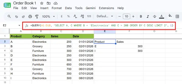
This does several things at once:
- Filters to only Electronics
- Filters again to sales above 200
- Sorts by sales in descending order
- Limits to the top 2 results
That’s a lot of work handled by one clean line of code.
Tips for Writing Better QUERY Formulas
Use proper syntax: SQL-like commands are case-insensitive, but consistent formatting makes formulas easier to read and debug.
Reference columns by letter: Use A, B, C instead of trying to reference by header name (unless your data structure supports named ranges).
Test incrementally: Start with a simple SELECT and WHERE, then add ORDER BY or GROUP BY once the basic filter works.
Watch for errors: Common mistakes include mismatched quotes, typos in column references, or forgetting to include the headers parameter when needed.
Remember the data range: Always include your header row in the data range if you set headers to 1.
Conclusion
The QUERY function transforms how you work with data in Google Sheets. Instead of spending time on manual filtering and sorting, you can write a formula that extracts exactly what you need in seconds. Whether you’re building a sales dashboard, analyzing survey responses, or pulling metrics for a report, QUERY handles the heavy lifting. Start with simple SELECT and WHERE statements, then layer in ORDER BY, GROUP BY, and LIMIT as your confidence grows. Once you’re comfortable with the basics, you’ll find yourself reaching for QUERY in almost every spreadsheet project.