If you use Google Sheets to manage a lot of data, you probably know how boring it is to copy and paste information from one spreadsheet file to another. The IMPORTRANGE function helps you do it easily. Sheets’ this function allows you to automatically pull data from one spreadsheet into another in real-time.

When it works it feels like magic. Your dashboards update on their own. Your whole team stays on the same page. When things break you usually end up staring at a very annoying #REF! error.

If your data has stopped flowing do not worry because it is easy to fix. Most IMPORTRANGE issues happen because of a simple mistakes. Here is how you can find and fix those IMPORTRANGE issues.

Why IMPORTRANGE Function Not Working?

Before going to the post, it is useful to understand why the function usually breaks. Here are the most common reasons:

Permision blocks is the first reason for failure. Since you are connecting two separate spreadsheet files, Google needs explicit permission to let the “destination” sheet read the “source” sheet.

Syntax slips is the second reason. If you miss the quotation mark or a misplaced comma it will break the entire formula.

Naming conflicts is the third reason. If you renamed a tab in your source sheet, the formula is now looking for a page that doesn’t exist.

Deleted or moved files is the fourth reason. If the source sheet was moved to a different folder or deleted entirely, the link is severed.

Fixes for IMPORTRANGE Function Not Working Issues

If your formula is acting up, try these steps in order:

1. The “Allow Access” Button

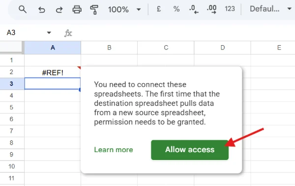
If you get the #REF! error when executing the function, hover your mouse over the cell. If a blue Allow Access button appears, click it. This is a security requirement from Google; the data won’t move until you manually authorize the connection.

2. Double-Check Your Syntax

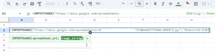
The formula must follow this exact structure: =IMPORTRANGE("spreadsheet_url", "sheet_name!cell_range")

Ensure the following in the formula:

• Wrapped both the URL and the range in double quotation marks.
• Used an exclamation mark to separate the sheet name from the cell range (e.g., Sheet1!A1:B10).
• Copied the full URL from the browser address bar.

3. Handle Spaces in Sheet Names

This is a common issue. If your Sheets’ tab name has a space in it (like Sales Data instead of SalesData), you must wrap the name in single quotes as seen below.

• Wrong: "Sales Data!A1:C20"
• Right: "'Sales Data'!A1:C20"

4. Verify Source Accessibility

Open the source spreadsheet in a new tab. If you can’t open it, the formula will not work. Check if the file was moved or if the permissions have changed.

Best Tips for a Proper Working of IMPORTRANGE Function

1. Keep names simple: Use clear, simple names for your spreadsheet tabs to reduce syntax errors.

2. Communicate changes: If you are the owner of a source sheet, let your team know before you rename a tab or move the file, as this will break formulas.

3. Document your links: Keep a small note or a “Control” tab listing which sheets are feeding into your main dashboard.

Conclusion

Learning these common issues and their solutions will help you fix the IMPORTRANGE function not working issue quickly. This will also help you maintain seamless data integration across your Google Sheets.