How to Create a Custom Search Box in Excel (Step-by-Step Guide)

Working with large spreadsheets is a time consuming task. Scrolling through hundreds or thousands of rows to find your data is a frustrating job and a waste of time. While Excel doesn’t come with a built-in search box feature like some other applications, you can build one yourself, and it’s easier than you might think.

Table of Contents

Why You Need a Search Box in Your Spreadsheet

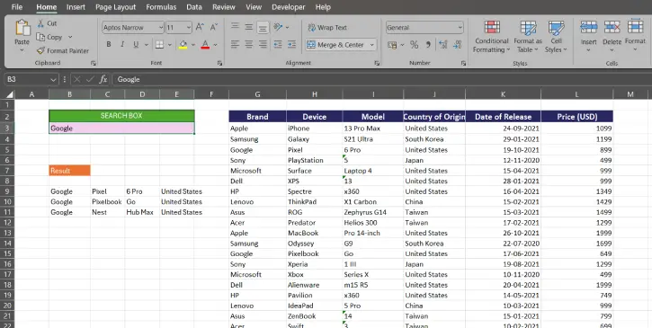
If you’re managing a big dataset, a search box can help you work with your spreadsheet quickly. Instead of using Excel‘s Find & Replace feature or manually scrolling through dataset, search feature gives instant results that update as you type.

Search box is particularly valuable when you’re sharing spreadsheets with colleagues who might not be comfortable navigating complex data structures.

How to Create a Custom Search Box In Excel Spreadsheet

In this example, I use Excel’s FILTER function to create a search box in spreadsheet. This function is available in Excel 2021+ and Excel 365. This method lets you create a real-time search experience without any macros or complex coding.

Step 1: Choose a cell where you want to enter the search term. In this example, cell B3. Above it, add a label in cell B2 that simply says “Search” so it’s clear what the field is for.

Step 2: Select a cell near your data (In this example, B9) and enter the below formula:

=FILTER(G3:J35, LEFT(G3:G35, LEN(B3))=B3,"Not Found")

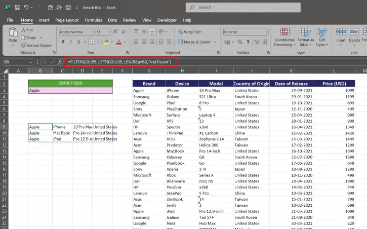
Note: Make sure to choose the range where your actual data lives (In this example, G3:J35). The B3 reference points to your search input cell—don’t change that.

Step 3: You have now created the search function in Excel. To test it, type something into cell B3. Your results appear instantly in columns G through J, and they update every time you change what’s in B3.

How this Search Function Works?

Let’s learn how this search function actually works:

The formula syntax in this example is: =FILTER(G3:J35, LEFT(G3:G35, LEN(B3))=B3,"Not Found")

Where LEFT(G3:G35, LEN(B3)) takes the first few characters of each cell in column G, matching how many characters you’ve typed in B3
=B3 compares those characters to what you typed
FILTER() displays only the rows where there’s a match
“Not Found” means if there are no matches, it shows nothing (you can change this to “Not Found” if you prefer)

For example,

Search for “Apple” → You’ll see every row that starts with “Apple”
Search for “App” → You’ll get broader results, including “Apple,” “Application,” anything beginning with “App”
Leave the search field empty → The full dataset displays (all rows from G3:J35)

Search for something that doesn’t exist → Nothing shows, which is exactly what you’d expect

Important Limitations of this Search Box

It searches one column by default. The formula as written only looks in column G (in this example). If you want to search across multiple columns, you’d need to modify it.

It matches from the start of text. This formula finds “App” at the beginning of cells, not “Apple” hidden in the middle. That’s usually a good thing, but it’s worth knowing.

The search is case-insensitive. “apple” and “APPLE” will both work the same way.

FAQ

Q: Can I search across multiple columns instead of just one?

A: Yes, but the formula gets more complex. You’d need to use SEARCH instead of LEFT and combine multiple conditions.

Q: Can I search for text anywhere in a cell, not just at the start?

A: Absolutely. Replace LEFT with SEARCH in your formula, and it’ll find matches anywhere within the text.

Q: Does this work with data in different sheets?

A: Not directly with this formula. You’d need to reference the other sheet in your range (like Sheet2!G3:J35), but the search box still needs to be on the same sheet as your formula.

Final Thoughts

Building your own search box in Excel is one of those small improvements that pays dividends, especially if you’re working with data regularly. It takes just a few minutes to set up, requires no programming knowledge, and makes your spreadsheet feel more professional and user-friendly.

The FILTER formula approach is clean, straightforward, and maintains full control over your data. Once you have it set up, you’ll wonder how you ever lived without it. If you’re sharing the spreadsheet with others, they’ll appreciate the convenience too—no more asking you where things are.