

SUMIF is one of the most useful functions in Google Sheets for adding up numbers based on conditions. Whether you’re tracking sales by product, filtering expenses by category, or summing amounts by date, SUMIF can do the heavy lifting for you. Let me walk you through how to use it with real examples.
How SUMIF Works: The Basic Formula
The syntax is straightforward:
=SUMIF(range, criterion, [sum_range])
Here’s what each part means:
- Range: The column you want to check (e.g., product names, dates, quantities)
- Criterion: The condition to match (e.g., “furniture,” “>100,” or a date)
- Sum_range: The column with numbers you want to add up (optional—if you skip it, it sums the range column instead)
A Simple Example of Using SUMIF in Sheets
Imagine you’re a freelancer tracking sales by product. You have:
- Column A: Product Names
- Column B: Product Category
- Column C: Sales
- To sum all sales for “F,” you’d use:
=SUMIF(A2:AI,"F",C2:C10)
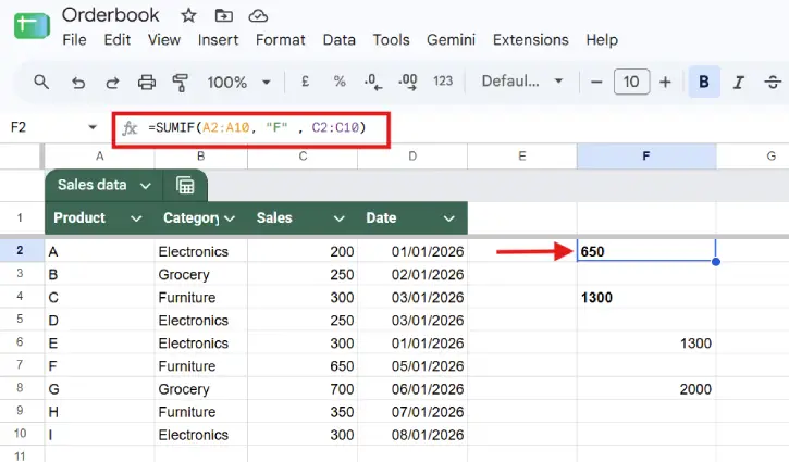
This searches column A for “Product F” and adds up the corresponding amounts in column C. Simple as that.
ALSO READ: How to Transpose Rows and Columns in Google Sheets (Two Methods)
SUMIF with Text: Finding Exact Matches
Text criteria work best for exact matches. If your data contains item names, client names, or categories, SUMIF finds them and sums the related numbers.
Exact Match Example
To sum furniture, in our example:
=SUMIF(B2:B10, "furniture", C2:C10)
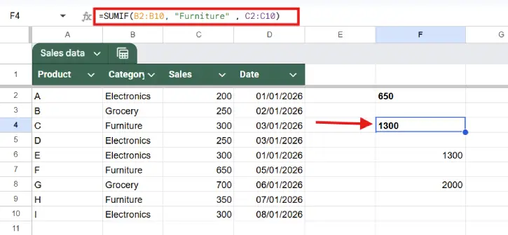
You can also put the criteria in a cell and reference it:
=SUMIF(B2:B10, B4, C2:C10)
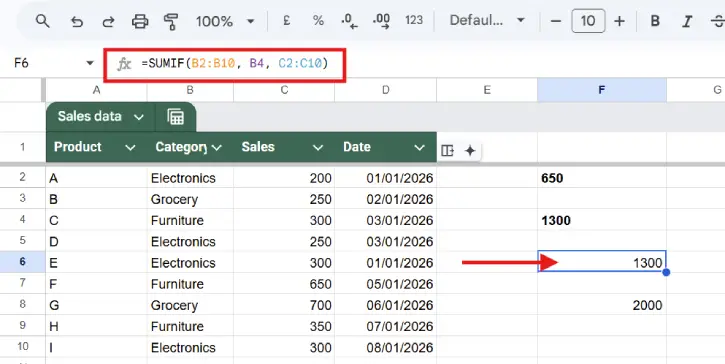
Where B4 contains “furniture.”
Excluding Items
To sum everything except furniture, use the “not equal to” operator:
=SUMIF(B2:B10, "<>furniture", C2:C10)
Or reference a cell:
=SUMIF(B2:B10, "<>"&B4, C2:C10)
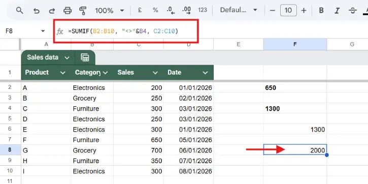
ALSO READ: Learn How to Use VLOOKUP in Google Sheets: A Practical Guide for Beginners
SUMIF with Wildcards: Partial Matches
When you need flexibility, wildcards let you match partial text. This is perfect for messy data or when you want to group similar items.
Use these wildcards:
- *= any number of characters
? = exactly one character
Wildcard Example
To sum all types of furniture:
=SUMIF(B2:B10, "*furniture*", C2:C10)
The asterisks mean find anything that contains the word ‘furniture.’
You can also combine wildcards with cell references:
=SUMIF(A2:A13,"*"&E1&"*",B2:B13)
Where E1 contains your search term.
SUMIF with Numbers: Comparisons and Thresholds
For numeric data, use comparison operators to sum amounts above or below a threshold.
| Formula | What It Does |
| =SUMIF(B2:B12,”<>200″,B2:B12) | Sum values that aren’t 200 |
| =SUMIF(B2:B12,”>200″,B2:B12) | Sum values greater than 200 |
| =SUMIF(B2:B12,”>=200″,B2:B12) | Sum values 200 or more |
| =SUMIF(B2:B12,”<200″,B2:B12) | Sum values less than 200 |
| =SUMIF(B2:B12,”<=200″,B2:B12) | Sum values 200 or less |
Number Example
Let’s say you’re tracking daily sales and want to sum all transactions above $200:
=SUMIF(B2:B12,">200",B2:B12)
You can also reference a cell:
=SUMIF(B2:B12,">"&E1,B2:B12)
Where E1 contains the threshold number (like 200).
SUMIF with Dates: Time-Based Conditions
Dates follow the same comparison logic as numbers. You can sum amounts from specific dates or date ranges.
Date Example
To sum deliveries before April 11, 2026:
=SUMIF(C2:C12,"<4/11/2026",B2:B12)
Or using the DATE function for clarity:
=SUMIF(C2:C12,"<"&DATE(2026,4,11),B2:B12)
Using TODAY()
To sum today’s orders
=SUMIF(C2:C12,TODAY(),B2:B12)
To sum past orders:
=SUMIF(C2:C12,"<"&TODAY(),B2:B12)
To sum future orders:
=SUMIF(C2:C12,">"&TODAY(),B2:B12)
SUMIF with Blank Cells
Sometimes you need to sum based on whether a cell is empty or filled. This is useful for tracking incomplete data.
=SUMIF(C5:C15,"",B5:B15) Sum if the cell is blank
=SUMIF(C5:C15,"<>",B5:B15) Sum if the cell is NOT blank
For example, to sum invoice amounts only for orders with a delivery date set:
=SUMIF(C5:C15,"<>",B5:B15)
This adds up column B only where column C has a date.
Handling Multiple Criteria (OR Logic)
SUMIF handles only one criterion at a time. To sum multiple items, add multiple SUMIF functions together.
Multiple Criteria Example
To sum both apples and oranges:
=SUMIF(A2:A12,"apples",B2:B12)+SUMIF(A2:A12,"oranges",B2:B12)
Or put the items in cells E1 and E2:
=SUMIF(A2:A12,E1,B2:B12)+SUMIF(A2:A12,E2,B2:B12)
This works like an OR statement—it sums values if the item matches apples or oranges.
Key Tips to Remember
Note that SUMIF only handles one criterion at a time. For multiple conditions using AND logic (all criteria must be true), use SUMIFS instead.
Also, keep your ranges the same size. If you use A2:A10 as your range, use B2:B10 as your sum_range (not B2:B100). This prevents confusion and errors.
Ensure to enclose plain text, operators with numbers, and wildcards in quotes: "apples", ">200", "*banana*". When combining operators with cell references, use an ampersand: ">"&E1, "<>"&E2. And, If you plan to copy your formula, lock the ranges with dollar signs: $A$2:$A$10

