If you’ve ever spent an afternoon manually deleting rows from a spreadsheet or copying formulas down hundreds of times, you know how soul-crushing it can be. The good news? Google Sheets has some seriously powerful formulas that can handle all that tedious work for you.

I’m going to walk you through five formulas that genuinely changed how I approach spreadsheets. Once you get the hang of these, you’ll wonder how you ever lived without them.

FILTER: See Only What Matters

Here’s the thing about FILTER—it’s like having a bouncer for your data. You tell it what rows to keep, and everything else disappears.

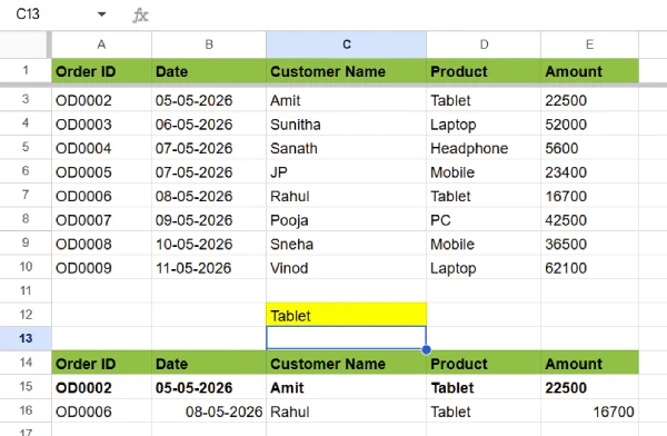
Let’s say you’re tracking sales data with columns for Name, Product, and Amount. You only care about sales over $1,000 because those are the deals worth celebrating. Instead of manually hunting through hundreds of rows, just use =FILTER(A:D, D:D>1000) and boom—only the big sales show up on your screen.

The best part? The rows stay in their original order, so your data doesn’t get scrambled. It’s automatic, clean, and saves you from the mindless clicking.

IMPORTRANGE: Connect Your Sheets Without Copy-Paste

Imagine having a “Team Budget” sheet that feeds automatically into your “Finance Report” without you lifting a finger. That’s what IMPORTRANGE does.

Instead of copying and pasting data every time something changes (which always happens at the worst time), you pull it directly with =IMPORTRANGE("the URL of your source sheet", "Team Budget!A1:D50"). The long string is just your Sheet ID from the URL—grab it once and forget about it.

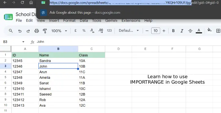
Now whenever the budget numbers update, your finance report reflects those changes instantly. It’s like having a live connection between your sheets.

ARRAYFORMULA: Apply One Formula to Hundreds of Rows

You know that painful feeling when you copy a formula down 500 times? ARRAYFORMULA eliminates that entirely.

Let’s say you want to add “Hello ” before every name in column B. Instead of copying =CONCATENATE("Hello ",A1) down forever, just write it once at the top with =ARRAYFORMULA(IF(A:A="","",CONCATENATE("Hello ",A:A))).

Now it automatically fills the entire column. New names added below? The formula covers them too. It’s like set-it-and-forget-it for your data transformation.

LET: Make Complex Formulas Actually Readable

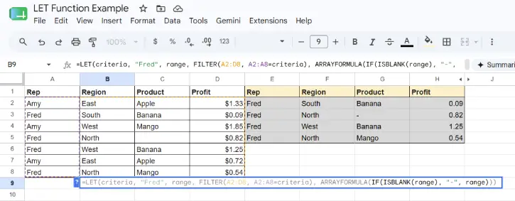
Complex formulas can turn into a nightmare of nested functions that nobody (including you) can understand three weeks later. LET fixes that by letting you create shorthand names for your values.

Instead of writing the same calculation twice in one formula—=IF(SUM(B2:B100)>1000, SUM(B2:B100)*0.1, 0)—you can do this:

=LET(total, SUM(B2:B100), IF(total>1000, total*0.1, 0))

You define “total” once and use it twice. Your formula is cleaner, faster, and way less likely to have errors. Plus, anyone reading it later (including future you) will actually understand what’s happening.

XLOOKUP: Find Data Without Wrestling with Formulas

XLOOKUP is what you wish VLOOKUP had been from the start. It’s simpler, more flexible, and doesn’t care about the order of your data.

Say you have a product list where column A has Product IDs and column B has Prices. To find the price of “P-453”, just use =XLOOKUP("P-453", A:A, B:B) and it returns the matching price instantly.

Better yet, you can reference a cell instead: =XLOOKUP(F2, A:A, B:B). Now you can drop any Product ID in F2 and it automatically pulls the price. No rearranging columns, no weird errors—just straightforward data lookup.

Conclusion

These five formulas are game-changers. They handle the grunt work so you can focus on actually analyzing your data instead of playing data janitor. FILTER and XLOOKUP help you find and organize what matters, IMPORTRANGE connects your sheets seamlessly, ARRAYFORMULA scales your formulas automatically, and LET keeps everything readable*

Start with whichever one solves your biggest spreadsheet headache, practice it once or twice, and you’ll be hooked. Your future self (and your sanity) will thank you.