

Today’s article reveals the most useful Excel Pivot Table shortcuts that every professional must know. These 20 keyboard shortcuts save time, improve accuracy, boost productivity, helps you summarize data in seconds, and bring clean, professional report.
Pivot tables transform raw data into a format that’s easy to analyze by letting you drag and drop fields to create custom summaries, cross-tabulations, and reports. And, the shortcuts significantly enhance productivity and improve overall performance of Excel use.
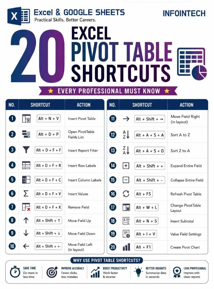
Table of Contents
20 Excel Pivot Table Shortcuts Every Professional Must Know
| NO. | SHORTCUT | ACTION |
| 1 | Alt + N + V | Insert Pivot Table |
| 2 | Alt + D + P | Open Pivot Table Fields List |
| 3 | Alt + D + F + F | Insert Report Filter |
| 4 | Alt + D + F + R | Insert Row Labels |
| 5 | Alt + D + F + C | Insert Column Labels |
| 6 | Alt + D + F + V | Insert Value |
| 7 | Ait + D + F + X | Remove Field |
| 8 | Alt + Shift + Up arrow | Move Field Up |
| 9 | Alt + Shift + Down arrow | Move Field Down |
| 10 | Alt + Shift + Left arrow | Move Field Left (in layout) |
| 11 | Alt + Shift + Right arrow | Move Field Right (in layout) |
| 12 | Alt + A + S + A | Sort A to Z |
| 13 | Alt + A + S + D | Sort Z to A |
| 14 | Alt + Shift ++ | Expand Entire Field |
| 15 | Alt + Shift +- | Collapse Entire Field |
| 16 | Alt + F5 | Refresh Pivot Table |
| 17 | Alt + W + L | Change Pivot Table Layout |
| 18 | Alt + N + S | Insert Subtotal |
| 19 | Alt + I + V | Value Field Settings |
| 20 | Alt + F1 | Create Pivot Chart |
What is a Pivot Table
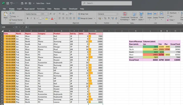
A pivot table is a data analysis tool in Excel that automatically summarizes, reorganizes, and aggregates large amounts of data from a source data range or database. It allows you to rearrange and filter data to see patterns, trends, and relationships without changing the original data.
Common Uses for Pivot Tables
Data Summarization: Quickly calculate totals, averages, counts, or other aggregations across large datasets without writing formulas.
Trend Analysis: Compare data across different time periods or categories to identify patterns (e.g., which products sell best in each quarter).
Cross-Tabulation Reports: Create two-dimensional summaries that show how data breaks down by two or more dimensions simultaneously.
Data Filtering: Isolate specific subsets of data (e.g., show only sales from the “North” region) to focus on relevant insights.
Comparative Analysis: Side-by-side comparisons of metrics across regions, time periods, departments, or other categories.
How to Create a Pivot Table in Excel (For Beginners)
- Select your data — Highlight the range including headers (e.g., A1:D100)
- Insert a Pivot Table — Go to Insert > Pivot Table (or use Alt + N + V shortcut)
- Choose location — Select whether to place it in a new sheet or existing sheet
- Drag fields — In the Pivot Table Fields pane, drag fields to Rows, Columns, Values, and Filters areas
- Summarize values — Right-click on values and choose your aggregation method (Sum, Average, Count, etc.)
Advantages of Pivot Tables
- Speed: Summarize thousands of rows in seconds
- Flexibility: Easily rearrange fields to view data from different angles
- No formulas needed: No complex Excel formulas required
- Interactive: Filter and drill down into specific data points
- Updates: Refresh the pivot table when source data changes
Conclusion
Pivot tables are one of Excel’s most powerful features for business analysis, financial reporting, and data exploration. Mastering these essential Excel Pivot Table shortcuts will help you boost your professional productivity, streamline your workflow, enables faster data analysis and improved performance.

