How to Use SORTBY Function in Excel to Sort Data in Ascending/Descending Order

If you have ever had trouble with Excel data—spending much time sorting manually, for example, student grades or trying to line up invoices by due date—you know how frustrating it can be. The SORTBY function, introduced in Excel 2021 makes sorting data much easier.

SORTBY allows you to sort one list based on the values in a completely different column in ascending or descending order. The best part of this Excel function is that it updates automatically whenever your data changes.

Table of Contents

How SORTBY Function Works and How to Use it

Imagine you are a school teacher. Column A contains the students names and Column B contains their exam marks. You want to see who the top performers are. SORTBY solves this instantly. It is simple. Click into a cell, type the formula, and press Enter:

=SORTBY(A2:A9, B2:B9, 1)

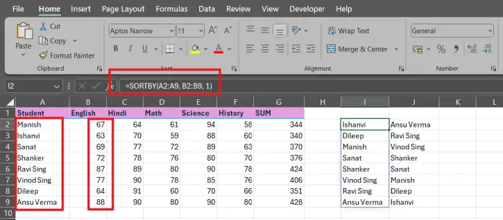
Where:

A2:A9: This is the list you want to see (the student names).

B2:B9: This is the engine that does the work (the exam marks).

1: This tells SORTBY to sort in ascending order ( to highest).

For descending order enter -1 [=SORTBY(A2:A8, B2:B8 -1)]

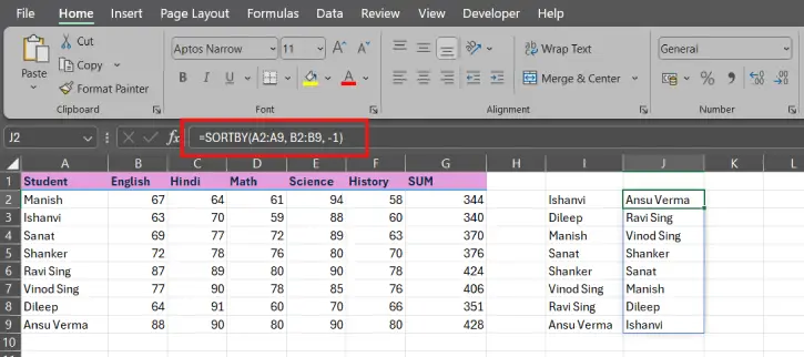
Once you press Enter the list will rearrange themselves based on those marks.

ALSO READ: How to Create a Custom Search Box in Excel (Step-by-Step Guide)

Where This Function is Useful in the Real World

SORTBY is not for teachers. It is a tool for almost any project:

Billing: Sort invoice descriptions by their date.
Sales: Rank your customers by how much they’ve spent.
Inventory: Organize products from lowest to stock levels.
HR: Sort employees by their start date or salary.
Planning: Order your to-do list by the closest deadline.

Note that if your formula does not work and getting parse errors, it is usually because of a few reasons:

The #NAME? error usually means you are using a older version Excel. The SORTBY function works with Office 2021 and later. If you get the #VALUE! error make sure your two ranges are the length. If your names go from A2 to A9, your marks must go from B2 to B9.

If you are getting the #SPILL! error, clear the cells underneath your formula so that data can spill down.

Pro Tips

You can put SORTBY inside functions like FILTER. For example, if you only want to see students who scored above 70 sorted from highest to lowest, enter the formula: =SORTBY(FILTER(A2:A8, B2:B8 > 70) FILTER(B2:B8, B2:B8 > 70) -1)

Final Thought

In the past sorting required risking the data order or spending a long time building a complex INDEX/MATCH formula. SORTBY removes the stress. Your original data stays where it is. The sorted list updates in time. It only takes one formula to set up. SORTBY is a faster and more organized way to handle your spreadsheets.