
Imagine you’re analyzing two variables—say, advertising spending and sales revenue. Google Sheets‘ Covariance function tells you whether these two things move together or in opposite directions. It’s the foundation for understanding relationships in your data, whether you’re doing financial analysis, scientific research, or business forecasting.
Think of covariance or COVAR function as a friendship meter for your data. Some variables are best friends (they go up and down together), some are frenemies (one goes up while the other goes down), and some barely know each other (no clear pattern).
Table of Contents
Understanding Covariance Function Results
When you calculate covariance, you’ll get one of three outcomes:
| Result Type | What It Means | Real-World Example |
| Positive covariance | Both variables increase or decrease together | Temperature rises → ice cream sales rise |
| Negative covariance | One variable goes up while the other goes down | Price increases → customer demand decreases |
| Zero or near-zero covariance | No clear relationship between the variables | Shoe size → test scores (no connection) |
How to Calculate Covariance in Google Sheets
Step 1: Set Up Your Data
Start with two columns of numbers you want to compare. Make sure your data is clean—no blank cells or text mixed in with the numbers.
Step 2: Click Your Target Cell
Navigate to the cell where you want your covariance result to appear. This is usually somewhere below or beside your data.
Step 3: Enter the COVAR Formula
Type this formula, replacing the ranges with your actual data:
=COVAR(A2:A6, B2:B6)
In this example:
A2:A6 = your first dataset (data_y)
B2:B6 = your second dataset (data_x)
Step 4: Hit Enter
Press Enter and Google Sheets will calculate your covariance value instantly.
A Practical Example of COVAR Function
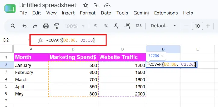
Let’s say you’re tracking monthly marketing spend (Column B) and website traffic (Column C):
| Month | Marketing Spend ($) | Website Traffic |
| January | 500 | 1200 |
| February | 600 | 1500 |
| March | 700 | 1800 |
| April | 550 | 1300 |
| May | 800 | 2000 |
You’d enter: =COVAR(B2:B6, C2:C6)
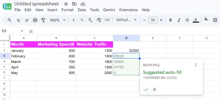
A positive result would confirm that higher marketing spending correlates with higher traffic. A negative result would suggest the opposite. Zero or near-zero would mean marketing spend doesn’t clearly affect traffic.
Important Note
Covariance isn’t the same as causation. Just because two things move together doesn’t mean one causes the other. Always investigate the story behind your numbers before drawing conclusions.
FAQ
Q: What’s the difference between COVAR and COVARIANCE in Google Sheets?
A: COVAR is the standard function in Google Sheets. Both terms refer to the same calculation—Google Sheets uses COVAR as its official function name.
Q: Can I use COVAR with more than two datasets?
A: No, COVAR only works with two datasets at a time. For multiple variables, you’d need to calculate covariance for each pair separately or use other statistical tools.
Q: What if my datasets have different lengths?
A: Your two ranges must have the same number of values. Google Sheets will return an error if they don’t match. Trim your data to equal lengths before calculating.
Q: Is a high covariance value always good?
A: Not necessarily. High covariance just means strong relationship—positive or negative. Whether that’s “good” depends entirely on your context and goals.
Q: Can covariance be negative?
A: Yes, absolutely. Negative covariance means the variables move in opposite directions, which is perfectly valid and often meaningful in analysis.
Conclusion
Covariance is a straightforward yet powerful tool for understanding how your data moves together. Whether you’re a business analyst tracking spending versus revenue, a researcher examining variables, or someone simply curious about data relationships, the COVAR function makes it easy to uncover these connections in Google Sheets.
The beauty of this function lies in its simplicity—just two ranges and one formula give you insight into whether your variables are partners, opponents, or strangers. While covariance won’t tell you why things move together, it’s the first step toward asking better questions about your data. Once you spot a relationship, you can dig deeper and uncover the real story behind the numbers. Start experimenting with your own datasets today. You might be surprised at what patterns emerge when you know where to look.