Ready to upgrade your Excel workflow? Start replacing your pivot tables with Excel’s new features GROUPBY and PIVOTBY. You’ll save time on setup and never worry about stale summaries again.

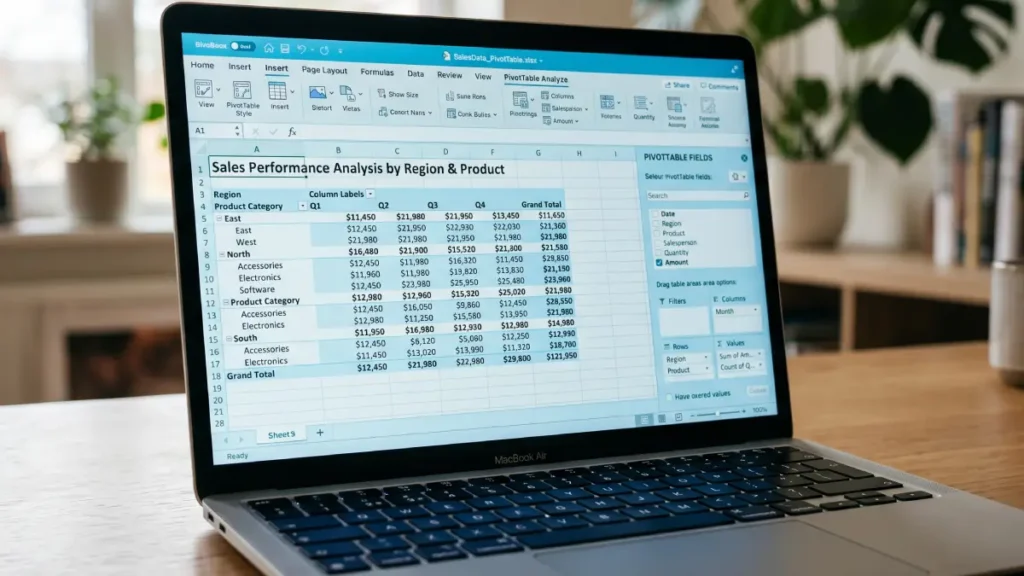
I spent years mastering pivot tables in Excel. Field lists, value settings, the whole dance—I had it down. But something always felt off. They worked fine for static reports, but the moment my work got serious, they became a liability.

Why I Stopped Using Pivot Tables

Here’s the thing about pivot tables: they don’t refresh automatically. You build a beautiful summary, share it with your team, and then the source data gets updated. Unless someone remembers to hit refresh—which they won’t—your summary becomes outdated. In a fast-moving spreadsheet where data changes constantly, that’s a deal-breaker.

There’s another problem too. Pivot tables live in isolation. You can’t easily chain them with other Excel functions, feed them into a FILTER, or use them as a live data source for charts. They’re powerful, but trapped in their own little world.

Then Microsoft quietly released GROUPBY and PIVOTBY as part of Office 365 update—two functions that do everything I was using pivot tables for, typed directly into a cell like any other formula.

GROUPBY: A Pivot Table That Actually Works

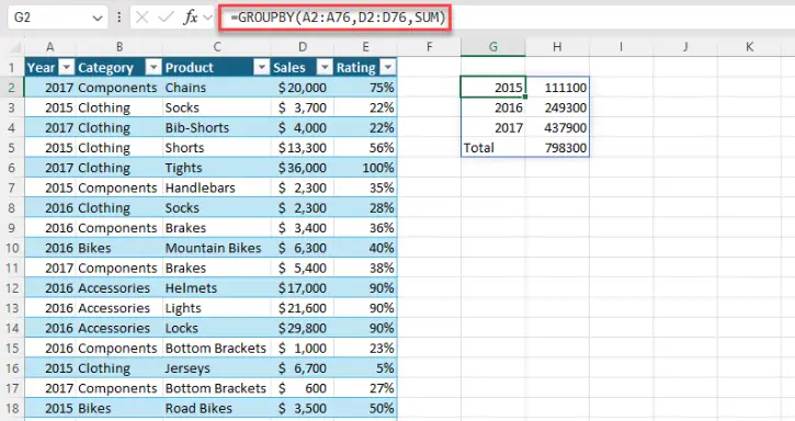
Think of GROUPBY as a pivot table that lives inside a formula. You give it three things: the column to group by, the column to aggregate, and the function to use. That’s it.

Let’s say you have a sales dataset and want total revenue by product category:

=GROUPBY(C2:C500, E2:E500, SUM)

Hit Enter, and Excel builds a complete summary table right in your sheet. Categories down one column, totals next to them. The best part? It updates the moment anything in your source data changes. No manual refresh. No stale numbers.

You’re not limited to SUM either. Use AVERAGE, COUNT, MIN, MAX, MEDIAN, or text aggregation functions (something pivot tables can’t do at all). You can sort the output, filter which rows get included, and control whether totals appear—all as arguments inside the formula. Tasks that would take extra steps or helper columns with pivot tables become one-line arguments.

PIVOTBY: Two-Dimensional Summaries Without the Headache

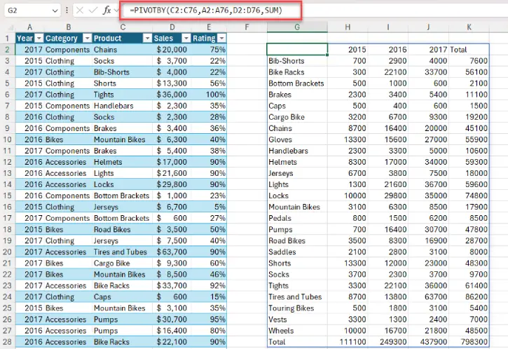
GROUPBY gives you one-dimensional summaries. For two dimensions—like sales by product and by month—you use PIVOTBY.

=PIVOTBY(C2:C500, A2:A500, E2:E500, SUM)

This builds a matrix with product categories down the left and months (or years, regions, whatever) across the top. The result is a live, dynamic array you can wrap in other functions, use as a chart source, or reference with spill notation. Your charts update when data updates. Your downstream formulas stay in sync automatically.

When to Still Use Traditional Pivot Tables

I’m not saying pivot tables are dead. They’re still better if you need slicers, timelines, or the ability to double-click a cell and drill into underlying rows. Pivot tables also handle automatic date grouping with a right-click—breaking dates into years, quarters, and months. With GROUPBY and PIVOTBY, you’ll wrap dates in YEAR() or MONTH() yourself.

Here’s the catch: these functions are Microsoft 365 only. If you’re sharing files with people on older Excel versions, the formulas won’t work for them.

ALSO READ: Excel Dynamic Filters: Set Up Once, Update Automatically

The Real Win: Staying in Control

What changed everything for me is this: I stopped thinking of my summaries as separate objects and started thinking of them as part of my formula logic. Charts pull live data from PIVOTBY results. Downstream calculations reference GROUPBY outputs. Everything stays in sync. Everything refreshes automatically. No manual interventions. No stale data.

If you’re building reports that run on the same dataset week after week and you expect the summary to just be right when the source updates, GROUPBY and PIVOTBY are the tools you’ve been waiting for.

FAQ

Q: Will GROUPBY and PIVOTBY work in my version of Excel?
A: Only if you have Microsoft 365. These functions won’t work in Excel 2021 or earlier standalone versions.

Q: Can I use GROUPBY and PIVOTBY with dynamic data ranges that change size?
A: Yes. If your data grows or shrinks, the formulas automatically adjust—no manual resizing needed.

Q: What if I need to drill down into individual rows from my summary?
A: Stick with traditional pivot tables for that feature. GROUPBY and PIVOTBY create summaries, not interactive drill-down objects.

Q: Can I filter or sort a GROUPBY result?
A: Yes. You can add FILTER and SORT as arguments inside the formula, or wrap the results with these functions afterward.

Q: Do these functions handle date grouping automatically?
A: No. You’ll need to wrap dates in YEAR(), MONTH(), or QUARTER() yourself to group by those dimensions.

Q: Can I combine GROUPBY and PIVOTBY with other formulas?
A: Absolutely. Since they’re formulas (not separate objects), you can chain them with FILTER, SORT, VLOOKUP, and anything else.

Conclusion

GROUPBY and PIVOTBY mark a real shift in how Excel handles data summaries. They’re faster to set up, automatically update, and integrate seamlessly with your existing formulas. If you’re on Microsoft 365 and tired of babysitting pivot tables, give them a try. Your future self—and your team—will thank you.