

If you’re managing product catalogs, customer feedback, or reports that span multiple countries, you know how tedious manual translation can be. You copy text, paste it into Google Translate, copy the result back—it’s time-consuming and error-prone.
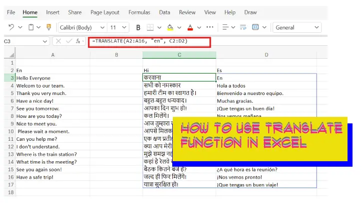
The good news? Excel has a built-in TRANSLATE function that handles all of this automatically. It connects to Microsoft’s Translation Services and supports over 130 languages. Best part? It’s just a formula away.
Table of Contents
How TRANSLATE Function Works in Excel?
The TRANSLATE function is straightforward. Here’s the syntax:
=TRANSLATE(text, [source_language], [target_language])
- text – The actual text you want to translate (or a cell reference)
- source_language – The language code of your original text, like “en” for English
- target_language – Where you want it translated to, like “fr” for French
Both language arguments are optional, but I’d recommend including them. Specifying the source language prevents Excel from guessing wrong on short phrases or ambiguous words.
Before you get start note that the TRANSLATE function only works with: Excel for Microsoft 365 (Windows and Mac), Excel for web, and Excel for mobile (iOS and Android). If you’re using the standalone versions like Excel 2024, Excel 2021, or Excel 2019, this won’t work. You’ll need a Microsoft 365 subscription.
How to Use Translation Formula in Excel?
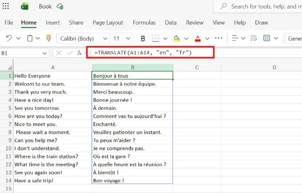
Let’s say you have product names in column A (rows 1-14) and you want them in French. Use this formula:
=TRANSLATE(A1:A14, "en", "fr")
Excel will translate all those cells at once and display the results in a dynamic array—meaning you don’t have to copy the formula down manually. All translations happen in one go.
If you only want to translate a single cell, just reference that one cell instead:
=TRANSLATE(B3, "en", "fr")
Important: Excel uses ISO language codes. Here are the most common ones:
“en” – English
“es” – Spanish
“fr” – French
“de” – German
“hi” – Hindi
“ja” – Japanese
“zh” – Chinese
“pt” – Portuguese
When you’re typing your formula, Excel’s IntelliSense feature (Formula AutoComplete) will suggest supported languages as you type. Just double-click the one you want and it automatically inserts the correct code.
How to Translate to Multiple Languages at Once in Excel
Here’s where things get interesting. You want the same product list in German, Spanish, and Italian. You can do this with one formula:
=TRANSLATE(A1:A14, "en", {"de","es","it"})
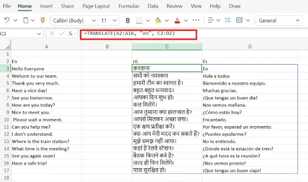
Or, if you prefer flexibility, put your language codes in cells (like C2:E2) and reference them instead:
=TRANSLATE(A1:A14, "en", C2:E2)
The second approach is better for real work because you can swap languages without editing the formula. Just change the codes in those cells and the translations update automatically.
Advanced: Dynamic Translation with a Dropdown
Here’s a practical setup for a real business scenario—like a customer service dashboard where agents need instant translations.
Step 1: Organize your data
- Put your source text in column A (e.g., A5:A20)
- Reserve cell C2 for a dropdown language selector
- Leave C5:C20 for the translated results
Step 2: Create a language lookup table
Make a simple table somewhere else on the sheet (like E4:F14) that maps language names to codes:
| Language | Code |
| German | de |
| Spanish | es |
| Italian | it |
| Hindi | hi |
| French | fr |
Step 3: Build a dynamic dropdown
In cell C2, set up Data Validation to reference your lookup table. Excel 365 users can use this formula to make it truly dynamic:
=TRIMRANGE($E5:$E20)
This automatically removes blank rows, so your dropdown stays clean as you add or remove languages.
Step 4: Write the master formula
In cell C5, combine XLOOKUP with TRANSLATE:
=TRANSLATE(A5:A20, "en", XLOOKUP(C2, E5:E20, F5:F20))
Now when someone picks “Spanish” from the dropdown, all your product names instantly translate to Spanish. Pick a different language, and everything updates. No manual work required.
Tips for Best Translation Results in Excel
Always specify the source language if you know it. Excel can auto-detect, but it’s less reliable with short phrases or words that exist in multiple languages. Being explicit prevents mistakes.
Use dynamic arrays when translating lists. Instead of copying a formula down row by row, reference the entire range (like B3:B18) and let Excel handle the spill automatically.
Keep your lookup tables organized. If you’re doing multi-language translations regularly, put your language codes in a separate sheet to avoid cluttering your main worksheet.
Test with ambiguous words first. If you’re unsure whether Excel will translate something correctly, try translating just that one phrase first before running the full formula.
The Takeaway
The TRANSLATE function transforms how you handle multilingual content in Excel. Instead of jumping between tabs and manual copy-pasting, you’ve got a formula that does the heavy lifting. Whether you’re translating a simple product list or building an interactive dashboard with live language selection, this tool saves hours of work.
If you’ve got Microsoft 365, there’s no reason not to use it. The learning curve is minimal, and the payoff is immediate—especially if your work touches multiple languages regularly.

